Choosing a Subset
Getting to Know Our Data Set
#Set CRAN mirror directly
options(repos = "https://cloud.r-project.org")

# Now try installing the package
install.packages("plyr")
##
## The downloaded binary packages are in
## /var/folders/q0/_0myr3tj3l986yfxrwn5xvbm0000gn/T//RtmpofBa5n/downloaded_packages## Linking to GEOS 3.11.0, GDAL 3.5.3, PROJ 9.1.0; sf_use_s2() is TRUE## ── Attaching core tidyverse packages ───────────────────────────────────────────────── tidyverse 2.0.0 ──
## ✔ dplyr 1.1.4 ✔ stringr 1.5.1
## ✔ forcats 1.0.0 ✔ tibble 3.2.1
## ✔ lubridate 1.9.3 ✔ tidyr 1.3.0
## ✔ purrr 1.0.2## ── Conflicts ─────────────────────────────────────────────────────────────────── tidyverse_conflicts() ──
## ✖ dplyr::filter() masks stats::filter()
## ✖ dplyr::lag() masks stats::lag()
## ✖ purrr::map() masks maps::map()
## ℹ Use the conflicted package (<http://conflicted.r-lib.org/>) to force all conflicts to become errors## -------------------------------------------------------------------------------------------------------
## You have loaded plyr after dplyr - this is likely to cause problems.
## If you need functions from both plyr and dplyr, please load plyr first, then dplyr:
## library(plyr); library(dplyr)
## -------------------------------------------------------------------------------------------------------
##
## Attaching package: 'plyr'
##
## The following objects are masked from 'package:dplyr':
##
## arrange, count, desc, failwith, id, mutate, rename, summarise, summarize
##
## The following object is masked from 'package:purrr':
##
## compact
##
## The following object is masked from 'package:maps':
##
## ozoneLets take a look at where the samples are from and get a little gauge of what is going on here, note: there are going to be some problems because we have yet to subset and clean our data, for example, some data points don’t have Lat and Long values:
#create a base map
background_map <- map_data("worldHires")

#load in the soil data
soil_data <- read_csv("SRDB_V5_1827/data/srdb-data-V5.csv")
## Warning: One or more parsing issues, call `problems()` on your data frame for details, e.g.:
## dat <- vroom(...)
## problems(dat)## Rows: 10366 Columns: 85
## ── Column specification ─────────────────────────────────────────────────────────────────────────────────
## Delimiter: ","
## chr (23): Entry_date, Author, Quality_flag, Contributor, Country, Region, Site_name, Site_ID, Manipul...
## dbl (62): Record_number, Study_number, Duplicate_record, Study_midyear, YearsOfData, Latitude, Longit...
##
## ℹ Use `spec()` to retrieve the full column specification for this data.
## ℹ Specify the column types or set `show_col_types = FALSE` to quiet this message.Now lets look at the columns the dataset contains:
##  [1] "Record_number"      "Entry_date"         "Study_number"       "Author"
##  [5] "Duplicate_record"   "Quality_flag"       "Contributor"        "Country"
##  [9] "Region"             "Site_name"          "Site_ID"            "Study_midyear"
## [13] "YearsOfData"        "Latitude"           "Longitude"          "Elevation"
## [17] "Manipulation"       "Manipulation_level" "Age_ecosystem"      "Age_disturbance"
## [21] "Species"            "Biome"              "Ecosystem_type"     "Ecosystem_state"
## [25] "Leaf_habit"         "Stage"              "Soil_type"          "Soil_drainage"
## [29] "Soil_BD"            "Soil_CN"            "Soil_sand"          "Soil_silt"
## [33] "Soil_clay"          "MAT"                "MAP"                "PET"
## [37] "Study_temp"         "Study_precip"       "Meas_method"        "Collar_height"
## [41] "Collar_depth"       "Chamber_area"       "Time_of_day"        "Meas_interval"
## [45] "Annual_coverage"    "Partition_method"   "Rs_annual"          "Rs_annual_err"
## [49] "Rs_interann_err"    "Rlitter_annual"     "Ra_annual"          "Rh_annual"
## [53] "RC_annual"          "Rs_spring"          "Rs_summer"          "Rs_autumn"
## [57] "Rs_winter"          "Rs_growingseason"   "Rs_wet"             "Rs_dry"
## [61] "RC_seasonal"        "RC_season"          "GPP"                "ER"
## [65] "NEP"                "NPP"                "ANPP"               "BNPP"
## [69] "NPP_FR"             "TBCA"               "Litter_flux"        "Rootlitter_flux"
## [73] "TotDet_flux"        "Ndep"               "LAI"                "BA"
## [77] "C_veg_total"        "C_AG"               "C_BG"               "C_CR"
## [81] "C_FR"               "C_litter"           "C_soilmineral"      "C_soildepth"
## [85] "Notes"
Great we have a bunch!
Visual Geographic Distribution of Points
#Lets color the points by biome, just to look:
ggplot() +
  #create the polygon map
  geom_polygon(data = background_map, aes(x = long, y = lat, group = group), fill = "lightgrey") +
  #add points to graph -> colored by biome
  geom_point(data = soil_data, aes(x = Longitude+rnorm(n=nrow(soil_data)), y = Latitude+rnorm(nrow(soil_data)), color=Biome), size = 0.5, alpha=.25, shape=4) +
  #project
  coord_fixed() +
  #graph text
  labs(title = "Map of Soil Sample Sites", x = "Longitude", y = "Latitude")
## Warning: Removed 383 rows containing missing values or values outside the scale range (`geom_point()`).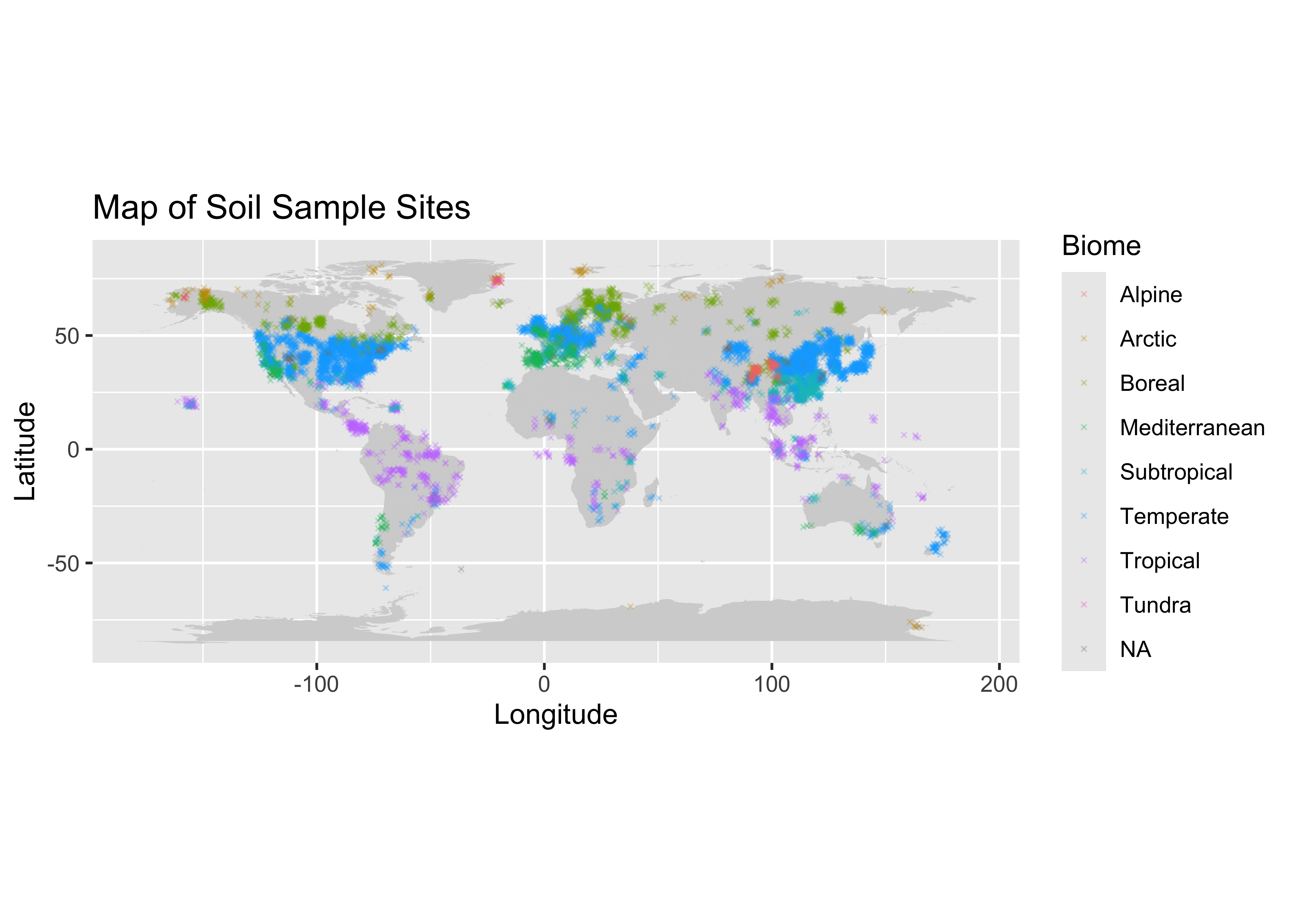 We can see some of the globe has a very sparse distribution of
information, I am thinking of subseting the data to get a better picture
of just one country.
We can see some of the globe has a very sparse distribution of
information, I am thinking of subseting the data to get a better picture
of just one country.
Distribution of Country Representation:
#getting the frequency of different countries:
country_counts <- count(soil_data, 'Country')
head(country_counts)
## Country freq
## 1 Africa 1
## 2 Algeria 2
## 3 Antarctic 2
## 4 Antarctica 7
## 5 Arctic 1
## 6 Argentina 20It seems like the frequency of datapoints per country is unsorted, we should look at them in order. I am starting to think we will want to look at some of the top represented countries for the next step of our exploratory analysis, because they will most likely have the most information (because there are more data points present), and hopefully they aren’t all NaN values.
Looking at the top 5 Most Represented Countries
#lets sort them to see the most frequent countries:
attach(country_counts)
country_counts_sorted <- country_counts[order(-freq), ]
head(country_counts_sorted)
## Country freq
## 22 China 3038
## 108 USA 2666
## 19 Canada 556
## 55 Japan 299
## 38 Finland 277
## 82 Russia 231We can visualize this with a bar plot:
# Select the top five
top_5 <- country_counts_sorted[1:5,]
y_top_5 <- top_5[['freq']]
x_top_5 <- top_5[['Country']]
#Plot with a bar chart
barplot(y_top_5, names.arg=x_top_5, horiz=TRUE, xlab = 'Frequency', main = 'Top 5 Countries Represented', las = 1, col = 'darkgreen')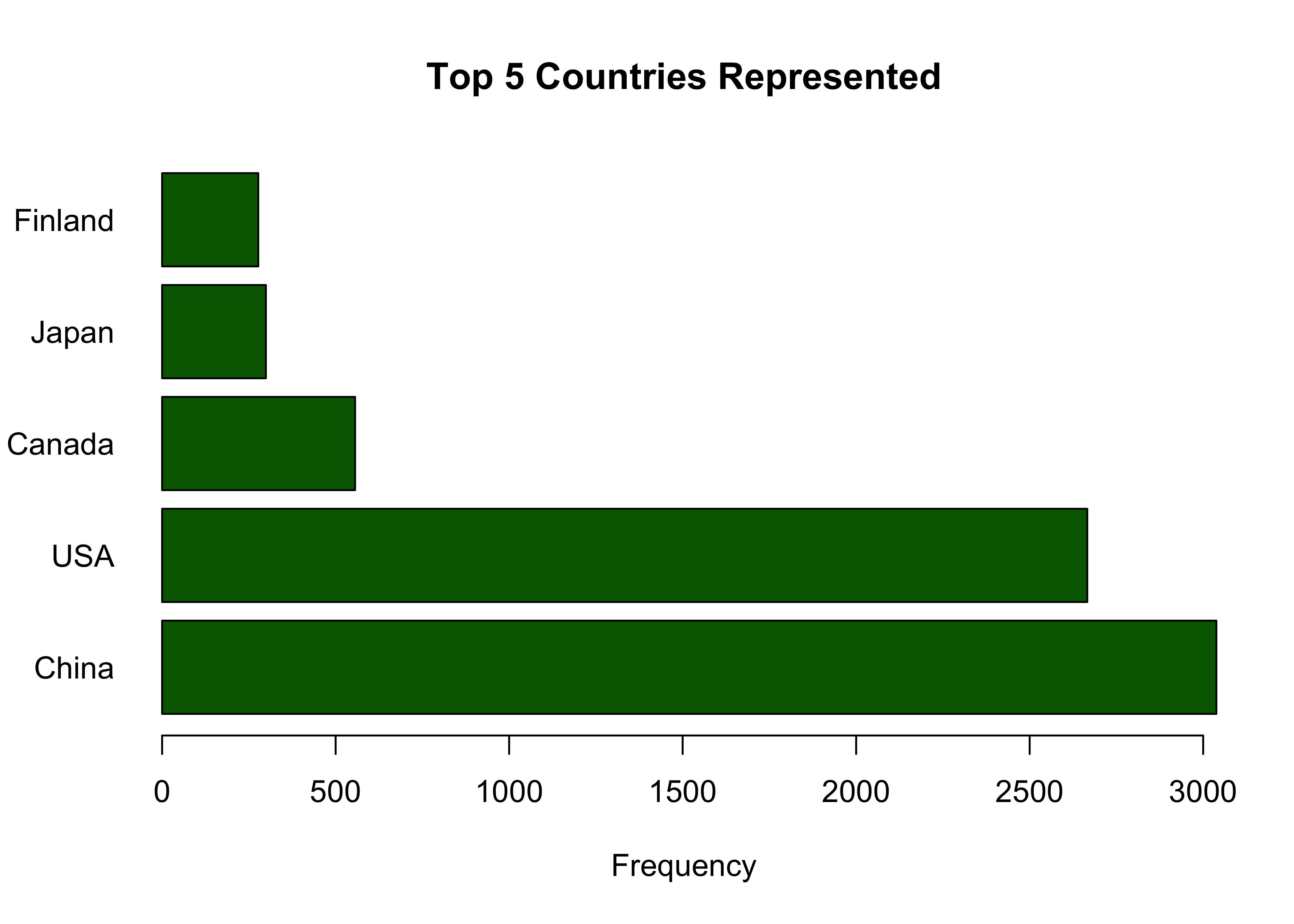 We see here that China and the USA make up a very large part of this
data set. I want to see which of the two has the lowest percentage of
missing values, then I will choose that subset of the data to look at
deeper and work on moving forward.
We see here that China and the USA make up a very large part of this
data set. I want to see which of the two has the lowest percentage of
missing values, then I will choose that subset of the data to look at
deeper and work on moving forward.
Subsetting China and USA & Quantifying Missing Data:
First we will only grab countries China and USA:
#select only China and USA
subset_list <- c("China", "USA")
china_usa = soil_data[soil_data$Country %in% subset_list, ]
And we can now see which has a lower proportion of missing values, we will also look at the distribution of quality flags for each group, because this will give us a better idea about the nature of information contained there:
china <- china_usa[china_usa$Country == "China",]
percent_missing_china <- mean(is.na(china)) * 100
percent_missing_china
## [1] 60.31677Lets now look at the percent missing from USA:
usa <- china_usa[china_usa$Country == "USA",]
percent_mising_usa <- mean(is.na(usa)) * 100
percent_mising_usa
## [1] 60.91479Great we can see that china has a slightly lower percentage of missing data.
Now let us look at the quality of data present, this data set makes it easier for us because they have included Quality flags which will gives us insight about the quality of data present in each observation.
Inspection of Quality Flags:
For reference we can describe each quality flag as follows:
Q0 default/none
Q01 estimated from figure
Q02 data from another study
Q03 data estimated–other
Q04 potentially useful future data
Q10 potential problem with data
Q11 suspected problem with data
Q12 known problem with data
Q13 duplicate
Q14 inconsistency
Let’s take a look at the distribution of flags for each group:
#count the occurences of each QF for each subset
usa_qf_counts <- count(usa, "Quality_flag")
china_qf_counts <- count(china, "Quality_flag")## Quality_flag freq
## 1 Q01 529
## 2 Q01,Q10 3
## 3 Q02 21
## 4 Q03 24
## 5 Q03,Q10 1
## 6 Q1 5
## 7 Q10 38
## 8 Q10,Q13 7
## 9 Q11 8
## 10 Q13 90
## 11 Q16 16
## 12 <NA> 1924## Quality_flag freq
## 1 Q01 529
## 2 Q01, Q11 15
## 3 Q02 7
## 4 Q03 37
## 5 Q1 90
## 6 Q10 10
## 7 Q11 1
## 8 Q11,Q12 4
## 9 Q11,Q14 3
## 10 Q12 1
## 11 Q13 3
## 12 Q15 2
## 13 Q16 12
## 14 <NA> 2324Alright we can pretty easily see that China has more data, and less potential problems with the quality of each observation.
Moving Forward with the China Subset:
The next step is cleaning the data, addressing missing values, and selecting our features of interest.
The first thing we will do is select data in China with quality flags = Q0 (or none), Q1, Q2, and Q3. I feel it would be potentially misleading or problematic to keep observations with the other QF’s, we will then save as a data set and move on to the cleaning and feature selection section!
ok_flags = c(NULL, "Q01", "Q1", "Q02", "Q03")
#subset based on the above criteria:
china_soil_respiration <- soil_data[(soil_data$Country == "China") & (soil_data$Quality_flag %in% ok_flags), ]
head(china_soil_respiration)
## # A tibble: 6 × 85
## Record_number Entry_date Study_number Author Duplicate_record Quality_flag Contributor Country Region
## <dbl> <chr> <dbl> <chr> <dbl> <chr> <chr> <chr> <chr>
## 1 276 2008-10-24 3653 Wang NA Q02 BBL China <NA>
## 2 277 2008-10-24 3653 Wang NA Q02 BBL China <NA>
## 3 278 2008-10-24 3653 Wang NA Q02 BBL China <NA>
## 4 279 2008-10-24 3653 Wang NA Q02 BBL China <NA>
## 5 280 2008-10-25 3653 Wang NA Q02 BBL China <NA>
## 6 281 2008-10-25 3653 Wang NA Q02 BBL China <NA>
## # ℹ 76 more variables: Site_name <chr>, Site_ID <chr>, Study_midyear <dbl>, YearsOfData <dbl>,
## # Latitude <dbl>, Longitude <dbl>, Elevation <dbl>, Manipulation <chr>, Manipulation_level <chr>,
## # Age_ecosystem <dbl>, Age_disturbance <dbl>, Species <chr>, Biome <chr>, Ecosystem_type <chr>,
## # Ecosystem_state <chr>, Leaf_habit <chr>, Stage <chr>, Soil_type <chr>, Soil_drainage <chr>,
## # Soil_BD <dbl>, Soil_CN <dbl>, Soil_sand <dbl>, Soil_silt <dbl>, Soil_clay <dbl>, MAT <dbl>,
## # MAP <dbl>, PET <dbl>, Study_temp <dbl>, Study_precip <dbl>, Meas_method <chr>, Collar_height <dbl>,
## # Collar_depth <dbl>, Chamber_area <dbl>, Time_of_day <chr>, Meas_interval <dbl>, …For fun we can look at the data we have that contains Lat, Long, and Annual Respiration values geographically.
Map of New Dataset:
#adding our map:
#Note the added random noise to see points clustered together at similar or the same testing sites
ggplot() +
  geom_polygon(data = background_map, aes(x = long, y = lat, group = group), fill = "lightgrey") +
  geom_point(data = china_soil_respiration, aes(x = Longitude+rnorm(n=nrow(china_soil_respiration)), y = Latitude+rnorm(n=nrow(china_soil_respiration)), color=Rs_annual), size = 2) +
  coord_sf(xlim = c(80, 130), ylim = c(10, 55)) +
  labs(title = "Map of Soil Sample Sites in China", x = "Longitude", y = "Latitude")
## Warning: Removed 24 rows containing missing values or values outside the scale range (`geom_point()`).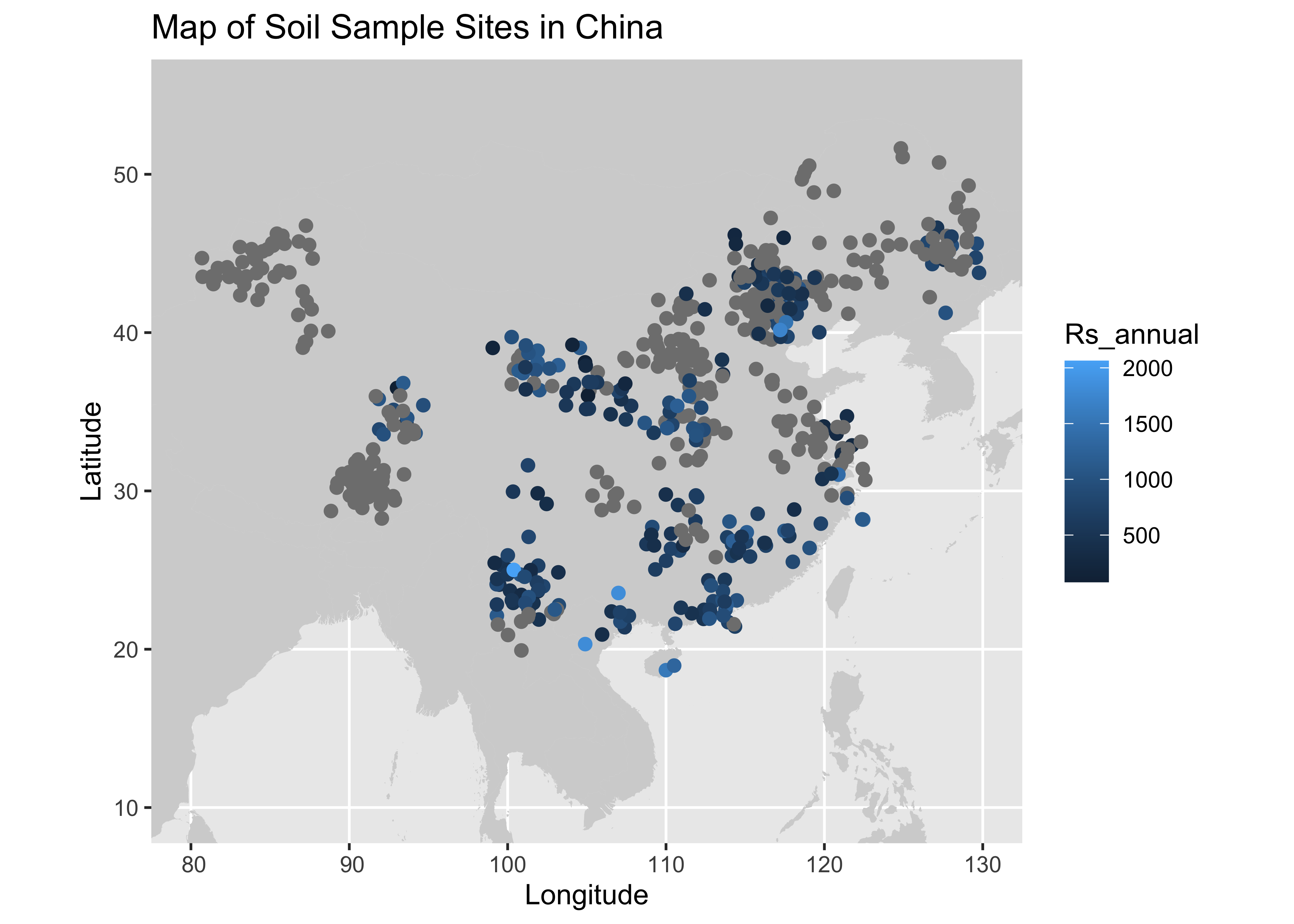
Now lets export this and move on to the next section: Data Cleaning and Feature Selection